One of the most mysterious events that happened in antiquity were total solar eclipses. Multiple interpretations were given to them, many of them sombre. Modern astronomical knowledge proved to be the key in making accurate predictions of many celestial mysteries, including eclipses. As an important byproduct, the mechanistic understanding helped demolish any supernatural interpretation of these events.
But aside from the (mis)interpretations of these events given in the past, I'd like to focus on their regularity. I would like to invite you to experience its modelling without knowing anything about celestial mechanics, which is a great opportunity to better appreciate the dangers that lack of knowledge carries in this sort of activities.
Eclipses happen rarely, but not too rarely so if you look at the Earth as a whole. A total solar eclipse occurs somewhere on Earth once every 18 months. But at a given location, it is estimated that they occur every 360–410 years, making them extremely rare events. This creates a severe problem which brings me to the main topic of this entry.
Before getting into it, let's further motivate this taking a quick step into the present. We live in a world surrounded by rare events. Think of pipeline failure, the nuclear industry, mining, aerospace, etc. Many times we have limited or corrupted data, and with limited knowledge of the causal patterns that produced the objects of study (say failure analysis), we enter a territory where conclusions are too uncertain and strongly dependent on the assumptions of our model. The two options that we have in such cases are: more data or better mechanistic models, or any combination of both. Logically both can be expensive or unfeasible. More data can help us narrow down model uncertainties, but more data with an incorrect model can be catastrophic. On the other hand, better models can be of great help but they require developing important theories. And sometimes, the modelling approach hits a wall.
Another issue in pipelines is that failure data is scarce by design. Pipelines are strategic assets where failure can have large consequences, so integrity and maintenance programs are designed to intervene before failure occurs. As a result, many pipelines are still operating when observation ends or when they are inspected, repaired, or replaced. We then know that their failure time is longer than the observed operating time, but we do not know the exact failure time. This is called right-censored data, and it is an important distinction from simply having few observed failures. One may think that studying repair actions can be used as a proxy, and inspection/repair decisions may themselves be informative because they depend on condition, policy, and risk. But it is also important to consider that not every detailed inspection may have been needed in the first place.
Let us go back to our eclipse example. Imagine that our knowldge of celestial mechanics is close to none. Then, statistical analysis becomes our main tool due the limited information we have.
We will assume that a given location experiences a total solar eclipse approximately once every 375 years, on average. Assuming that we do not know this number, we can do statistical analysis by treating the events as purely random, which is a strong and incorrect assumption as you may suspect.
But still, if the true time between events is 375 years, one question that we me ask is: how much data do we need to estimate this rate plus minos 10% error? How many events do you need? How long in the past do we need records?
The model
We'll model the arrival of each eclipse as a Poisson process. A Poisson process is the only memoryless process, that means that it models each event as independent of any other that had happened in the past. Therefore the probability of seeing an eclipse does not change by observing an eclipse. This is a very strong and wrong assumption about the process that generates the eclipses, but we will use this deliberatively wrong assumption as an instructive baseline.
For a Poisson process, the parameter \(\lambda\) is the event rate. In this case,
The number of eclipses observed over a period of \(t\) years is then
The probability of observing \(k\) eclipses during those \(t\) years is
Equivalently, the waiting time \(X\) between eclipses follows an exponential distribution:
We'll use this simplified model that assumes a purely random arrival process to show what happens with rare events. Eclipses are not truly random Poisson events, but we will use this incorrect model to illustratate the difficulty of inferring the frequency of rare events from limited observations.
To make the problem concrete, we will simulate one location. We'll start from an ssumed most recent event, and from that year we draw nine successive waiting times from the exponential distribution above. The simulation produces the following observation history:
| Event | Year | Delta from previous event |
|---|---|---|
| 1 | 2002 | — |
| 2 | 1627 | 375 years |
| 3 | 1441 | 186 years |
| 4 | 1304 | 137 years |
| 5 | 521 | 783 years |
| 6 | 115 BCE | 635 years |
| 7 | 491 BCE | 376 years |
| 8 | 782 BCE | 291 years |
| 9 | 1190 BCE | 408 years |
| 10 | 1408 BCE | 218 years |
Let \(k_i\) be the number of events observed during period \(i\), whose duration is \(t_i\). The likelihood of each observation is
Because the observations are independent, the likelihood of the complete data is the product of the individual likelihoods:
The logarithm is a monotonically increasing transformation. Therefore, it preserves the value of \(\lambda\) that maximizes the likelihood, while turning the product into a sum. The log-likelihood is:
Taking the derivative with respect to \(\lambda\),
Which gives us the maximum-likelihood estimator (MLE):
In other words, the Poisson MLE is the total number of observed events divided by the total observation time.
For our simulated history, we observed ten event dates, which define nine waiting intervals, over a total span of \(t=3{,}409\) years. Since the most recent event was chosen as the endpoint, the appropriate count for the waiting-time estimate is \(k=9\) not the 10 events we observed. The actual observations were the time between observations. Substituting these values gives:
The corresponding estimated mean interval between events is
This estimate is close to the generating mean interval of 375 years. However, that agreement alone does not establish precision, as it may have been that by random chance we happened to land on a MLE close to the true parameter.
Then the question is how confidently an observer, without knowing the generating parameter, could estimate the rate from this history. The key here is without knowing the generating parameter.
So we are stress testing this model thoroughly from within, i.e., we are still assuming our wrong model is true. How do we define confidence interval?
We can estimate a confidence interval using the exact sampling distribution of the exponential model. Let the nine observed waiting times be \(X_1,\ldots,X_9\), each modeled as
Their total is
The chi-squared distribution appears after nondimensionalizing the waiting times: multiplying by the unknown rate removes the time unit. The detailed change of variables derivation is given in the Appendix. The result is
where \(S=\sum_{i=1}^{n}X_i\) and \(n=9\), so the degrees of freedom are \(2n=18\). The distribution of \(2\lambda S\) is known even though \(\lambda\) is unknown, making it a pivot. We can therefore choose the central 90% of its chi-squared distribution and solve the resulting inequality for \(\lambda\). This gives an exact \(100(1-\alpha)\%\) confidence interval:
For a 90% confidence interval, we set \(\alpha=0.10\):
This exact interval is preferable to a Central Limit Theorem approximation here because we have only nine waiting intervals and the exponential distribution is strongly skewed. We can also invert the endpoints to obtain a confidence interval for the mean waiting time \(1/\lambda\).
Using the chi-squared quantiles \(\chi^2_{18,0.05}\approx9.390\) and \(\chi^2_{18,0.95}\approx28.869\), the exact interval is
Equivalently, the mean waiting time lies approximately in
For comparison, a normal approximation uses the estimated standard error
Using the 90% normal critical value \(z_{0.95}\approx1.645\), the corresponding Wald interval is
This gives a mean waiting-time interval of approximately \([244.6,\ 838.5]\) years. The normal interval is somewhat wider after inversion, while the exact interval is preferable because it respects the skewed sampling distribution and the small sample size.
Let us reflect on these results
First, we inverted the confidence interval endpoints to estimate the mean waiting time \(1/\lambda\). This transformation makes the interval asymmetric. The exact interval is approximately 236–726 years, while the normal approximation gives approximately 245–839 years. Note how the width of the CI changes and how it has a different coverage.
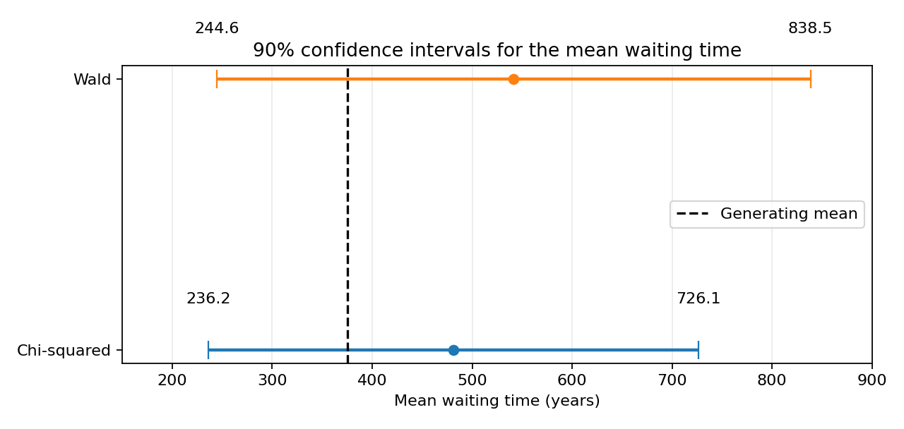
Figure: Confidence intervals for the parameter \(1/\lambda\) under two different interval constructions. Notice how the same data, analyzed using two different methods, produces different CIs.
Second, it is important to say that in this frequentist framework, a 90% confidence interval does not mean that there is a 90% probability that this particular interval contains the parameter. In repeated samples, the interval-construction procedure is designed to contain the true parameter in approximately 90% of cases. Our single interval is one realization of that procedure.
However, in reality we do not have the privilege of "running the simulation multiple times". The eclipses that happened, happened, and they are not within our control. But if we needed more data we could seek records of eclipses observed at other locations and see what additional information they provide. More on that later.
Going back to this result, this level of uncertainty is difficult to tolerate. Imagine you wanted to predict the next eclipse, and all you could say according to the data and your strong assumptions is that it should happen sometime between approximately 2243 and 2733. The predictive power is low. Moreover, even if the model were accurate, the uncertainty would be so large that the result would not be practically useful.
What can we do now
We can estimate how the confidence interval width changes as the number of observations increases. Knowing that the generating mean waiting time in this simulation is 375 years, we can search for the minimum number of observations that produces an interval width we consider tolerable.
Because the total observed time \(S\) varies from sample to sample, there is no single interval width determined by \(n\) alone. A simulation lets us study the sampling behavior directly:
For a candidate number of intervals \(n\), the exact confidence interval for the event rate is
After inverting the endpoints, the corresponding interval for the mean waiting time \(\mu=1/\lambda\) is
Its width is therefore
The total observation time \(S\) is random, so \(W(n,S)\) is random as well. We can nevertheless use the expected total time \(E[S]=n/\lambda_0\), where \(\lambda_0=1/375\), to get a rough planning approximation:
This approximation is useful for planning, but simulation is better for understanding the full distribution of possible interval widths:
- Choose a candidate number of waiting intervals \(n\).
- Simulate many datasets from \(\operatorname{Exponential}(1/375)\).
- Compute the exact confidence interval for each dataset.
- Measure the average, median, or upper percentile of the resulting interval widths.
- Increase \(n\) until the interval width meets the practical requirement.
This reframes the question from “What is the confidence interval from this one history?” to “How much data would this method need before its uncertainty became useful?”
Let us define a useful target: a 90% confidence interval whose total width for the event rate is no more than 10% of the true rate \(\lambda_0=1/375\). Using the exact chi-squared interval and the expected observation time \(E[S]=n/\lambda_0\), we search for the smallest \(n\) satisfying
Solving this equation we find that we re require
waiting intervals for a 90% level of confidence. At a mean interval of 375 years, the expected observation time is
Much longer than the span of human written and instrumental records. To estimate the event rate to this level of relative precision, we would need more than four hundred thousand years of observations at a single location. One possible solution is to use more location records, but we need to be careful that those eclipses are truly independent. We don't want to use data from location affected by the same eclipse to count as more independent evidence towards refining our estimate.
We also need to consider the case of what happened if an eclipse was not recorded, so we have gaps in our eclipse data? Or what happens if the eclipses records are subject to some random source of variations? Two important things to consider that we'll leave for another day.
Confirming the result with a replication study
To assess the result across repeated samples, we'll simulate 1,000 random seeds to compute the empirical CI width using the same rate \(\lambda_0=1/375\). The first replication gives
The exact 90% confidence interval is
Its width relative to the true rate is
or approximately \(9.74\%\). This particular simulated interval is therefore within the 10% target. It does not guarantee that every dataset with \(n=1{,}085\) intervals will meet the target: the total observation time is random, so the interval width varies from sample to sample.
Across all 1,000 replications, the mean MLE is approximately
and the median MLE is approximately
The mean and median relative confidence interval width are approximately \(9.99\%\). Of the 1,000 simulated intervals, approximately \(52.3\%\) are within the 10% target. Approximately \(88.9\%\) contain the true rate, close to the nominal 90% coverage.
The replication procedure can be repeated for different values of \(N\). The plot below shows the relative confidence-interval width as the number of waiting intervals increases. Each point uses 1,000 simulated datasets. The shaded band contains the 10th through 90th percentiles for each \(N\).
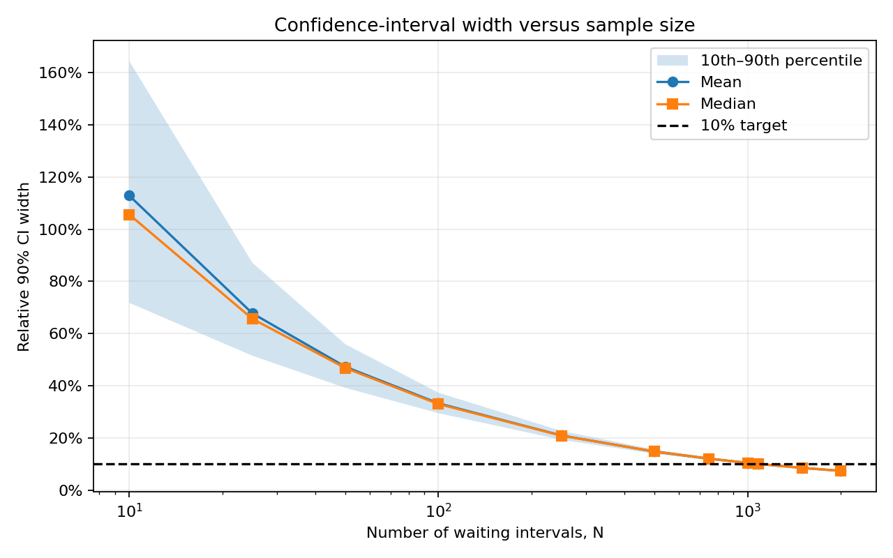
The typical interval width decreases as \(N\) increases, approximately following a \(1/\sqrt{N}\) relationship. The spread across replications also shows why a target based on expected width is not a guarantee for an individual dataset.
Conclusion
More than 400,000 years of observations would still leave a simple statistical recurrence model with limited predictive value. The problem is that historical frequency alone cannot reveal the causal structure governing eclipse timing.
Modern eclipse prediction became possible because celestial mechanics supplied that highly predictive structure required for this problem, which allows us to predict total solar eclipses far ahead in the future (and the past as well) with precision lower than minutes.
How does any of this apply to pipeline integrity?
Pipeline integrity is not fully deterministic or mechanistic. It is not fully aleatory either. It sits somewhere in the middle. Things to consider about pipeline failure:
- Pipeline failure is rare
- Pipeline failure is multifactorial
- Our understanding of the state of the pipe is not fully well determined (think of stresses, strain state, etc)
- Our physical understanding of failure modes is not complete (for cracks for example, CorLAS? MAT-8? Other?)
- Our knowledge of pipeline properties is incomplete (exact wall thickness at given location? Exact morphology of a feature? Exact SMYS/UTS? Etc.)
- Using historical data to determine pipeline failure is misleading due to the uncertainty of historically derived parameters, and due to the multifactorial process that produces failure.
Statistical inference and mechanistic modeling complement each other. The problem is relying on historical frequency data alone when failures are rare and heterogeneous, while ignoring the mechanistic pattern that produces the data.
I leave the floor open. I have a few more things to say and I might update this entry in the near future. In pipeline integrity, the answer is usually not better models or more data, but better models that determine which data are informative and how they should be combined.
Appendix: Nondimensionalization and the chi-squared pivot
The exponential waiting time \(X_i\) has rate \(\lambda\), so its numerical value depends on the unit used for time. The trick here is that a simple change of variable removes that unit, and by doing so it removes its dependency on the parameter.
We use the conventional factor of two and define
Since \(X_i\sim\operatorname{Exponential}(\lambda)\), the change of variable formula gives
This is the density of a chi-squared random variable with two degrees of freedom, so \(Y_i\sim\chi^2_2\). Because the waiting times are independent, the \(Y_i\) are independent. Their sum is therefore chi-squared with degrees of freedom that add:
This is the pivot used in the confidence interval. Its reference distribution is known and does not depend on the unknown rate once the data are combined with the parameter in the expression \(2\lambda S\).